Levitating Ball in Tube PID Control Systems Demo
Advisor(s): Dr. Reza Rashidi, Dr. Aaron Estes
Team #31
Team Name: Levitating Ball in Tube PID Control Systems Demo
Section: B
Final Memo MAE 494
Date: 05/07/24
Prepared by:
Ethan Fort
Shardul Saptarshi
Bryce Zilch
Kody Zachgo
Evan Fanara
Mechanical and Aerospace Engineering Senior Design Project
The State University of New York at Buffalo
Buffalo, New York
Fall 2023
We would like to express our gratitude towards Dr. Estes for his support and contribution towards our senior design project. His generous sponsorship, technical guidance, and thorough involvement throughout the project have played a major role in the design process. Additionally, we would like to extend our appreciation towards Dr. Estes’ trust in our abilities and his belief in the project’s potential. We look forward to continuing to build our relationship with him as we move into the upcoming phases of the project. Also, we would like to thank Dr. Rashidi for fielding all of our questions regarding the project. The timely and insightful answers have helped us along the way.
Table 1. General Project Overview 9
9.1 Modeling, Fixtures, & Housing 27
13.2 Knob adjustable sampling rate 40
13.4 Mapping the control output to the servo motor angle 41
Extending upon the previous conceptual framework, a prototype is introduced for an educational demonstration of a levitating ball-in-tube PID control system. This memo serves as a general review of design, an in-depth look at the design methodology, and standards followed.
Construction for this project can be simply divided into two sections. One is hardware which includes the product housing design, subsystem integration, and prototype testing. The other branch is software development which includes controller incorporation, UI/Data interface design, and mathematical model development. In effect this makes a ‘simple’ system with the goal control the position of a ball in a tube using a PID control system and another acting as the educational interface to teach students about control systems
To represent the aforementioned system we present an updated version of our design from last semester, including drawings and component views. Regarding the methodology, a discussion of each component is presented, the background for the mathematical model is introduced, and initial data is presented from model fitting. Initial rapid prototyping work thus far is presented, including 3D models, code, and data.
Regarding the project, I am a part of the software/modeling team. On that side of things, Shardul and I have focused on the code that runs the system, the mathematical background of the project, and the user interface. I have made significant contributions to the Arduino code, specifically the code running the controller, to subsystem integration, and I have done significant research to find an adequate approach to modeling. For the midterm memo, I completed the abstract, introduction, system design review, table of product specifications, engineering standards, and the software section of the design methodology. For the final memo I completed the ‘Hardware’ section of the implementation section, as well as the ‘Arduino code’ section. I also contributed to the validation section and completed the recommendation section.
Being part of the hardware design team, I helped with reviewing ideas for the designs of the 3-D prints and researching the means we will use for the final production of our prototype. I helped additionally in keeping the team on track so we don't get caught up in ideas and problems that were not applicable or insignificant so we remain at the current pace we're at. I also helped communicate with the sponsor so we are able to deliver a quality product that they would be satisfied with and the difficulties we encountered and had to remodel due to the sponsor's requests. For the memo, I helped review each section of the memo as well as the hardware portion of the memo.
As a member of the software team for this project, I have helped design the proportional controller using Arduino IDE code. Along with Ethan, I engaged in hardware debugging and testing, which involved circuit building, soldering, and system response analysis. For this memo, I helped develop the analysis section. I articulated our analysis strategy for the various tests that we conducted. I also wrote the modeling section of the design methodology, and included the methods we used to identify the future steps our team needs to take in order to develop an accurate system model. In addition, I updated the methodology to include my work on the physical user interface and MATLAB software.
As a member of the hardware team for this project, I helped design the 3-D printed hardware components for the project based on the dimensioning of traditional hardware used. I also player a large role in the design and fabrication of the main acrylic housing and its fixtures. I have additionally participated in hardware testing to identify problems with the hardware, and worked to create iterations of the hardware and new ideas for hardware that solve developing issues. For the midterm memo I wrote the hardware section of the methodology, and the modeling and design section for the design review. For the final memo I helped write the conclusions, validation, and implementation sections.
As a member of the hardware team for this project, I helped generate prototype ideas and then subsequently modeled each one in Autodesk Inventor. Throughout the iterative process, I worked with the team to refine each design and modeled new iterations after implementing the design changes. I have additionally participated in hardware testing to identify problems with the hardware and worked to help solve problems with each prototype. For this memo, I performed the Finite Element Analysis to identify the structural challenges with specific prototypes through the design process.
Demonstrations are an important part of any educational curriculum. They allow students to form the connection between the theory they learn in formal lectures, and real life where they will need to apply this knowledge practically. Our group (Group 31) proposes a control system that levitates a ping pong ball in a tube using PID control, with the foundational purpose of being used in an educational setting for students with any background. Control systems are not trivial to understand and visualize in a practical sense while learning the theory. This product will provide students with a hands-on experience, and interactive experience with a control system, that will help them learn the concepts, and also provide motivation for what they are learning in the classroom. It shall give students a feel for control theory, and any hardware in the system. As such, all design decisions were made with students in mind, to deliver a functional and effective system.
The project sponsor, Dr. Estes of the MAE department, will use this system as a demonstration for his classes in digital controls and mechatronics. He offered an exceptional project proposal which laid a strong foundation from which to begin the design process. This product has been funded by the MAE department, highlighting its educational importance.
The decision-making processes driving our approach prioritize educational effectiveness and user experience. Every design choice is made through the lens of student engagement and comprehension. The system must not only be functional but also robust, aesthetically pleasing, and efficient to meet the needs of its educational environment. Functionality and performance will be evaluated through system accuracy, speed, durability, and from the student side the user experience.
Overall, our goal is to deliver a fully functional educational demonstration that can be used in the classroom and for MAE department showcasing events. To do this we need to both deliver the hardware and software that controls and maintains the position of a ping-pong ball, as well as the front-end tools and interfaces to display to users of any background how this is possible.
From the proposal it was stated that the system shall act as a standalone educational demonstration utilizing a microcontroller, and does not necessarily have to be connected to a PC/Laptop, however, it shall have the ability to connect via USB so that any relevant data can be recorded and displayed. To fulfill the standalone requirement the system requires an external power supply that provides power to the entire system.
In normal operation, the system needs to make a ping pong ball hover at an adjustable height by controlling a fan at the base of a clear and graduated tube of around ~ 2 ft in length. An infrared sensor, with an adjustable sampling rate (Up to 20 Hz), needs to monitor the ball's height and send the measurements to the controller for it to make necessary adjustments to the actuator. The control algorithm will be using PID control and tuned based on experimental data. The actuator is a 12V stepper motor that controls a flap that restricts or allows airflow to a 12V computer fan set at a constant speed. As the flap moves it will change the airflow through the fan, therefore changing the ball position due to the resulting pressure change on the ball. The microcontroller's output needs to be scaled by three adjustable gain values, which should be constrained to reasonable levels. This will allow a user to adjust the gain parameters and explore what happens to the response, in a realistic environment. The control system software will account for integrator windup, and saturation, and will have an automatic shutoff to enhance robustness and reduce wear. For its educational purposes, we will be delivering an interactive UI that will allow students to simulate mathematical models for comparison to real system operation, a way to self-tune the controller based on experimental data, and a display that updates in real-time to show system behavior.
Product Features Operational Features
Educational Features
Physical Dimensions
| Product Performance Electrical Specifications
Sharp GP2Y0A21YK0F Specs [1] [5]
Controller Specs
Servo Specs [2]
System Performance
|
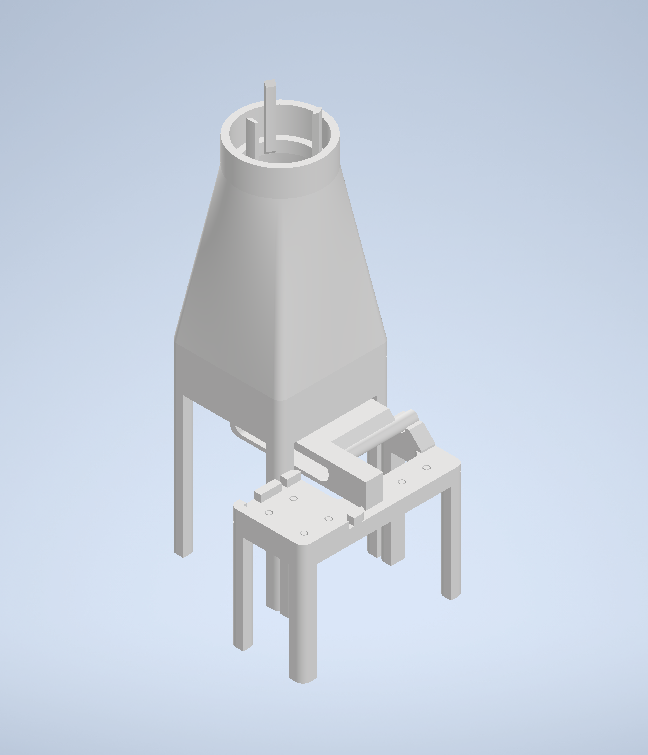
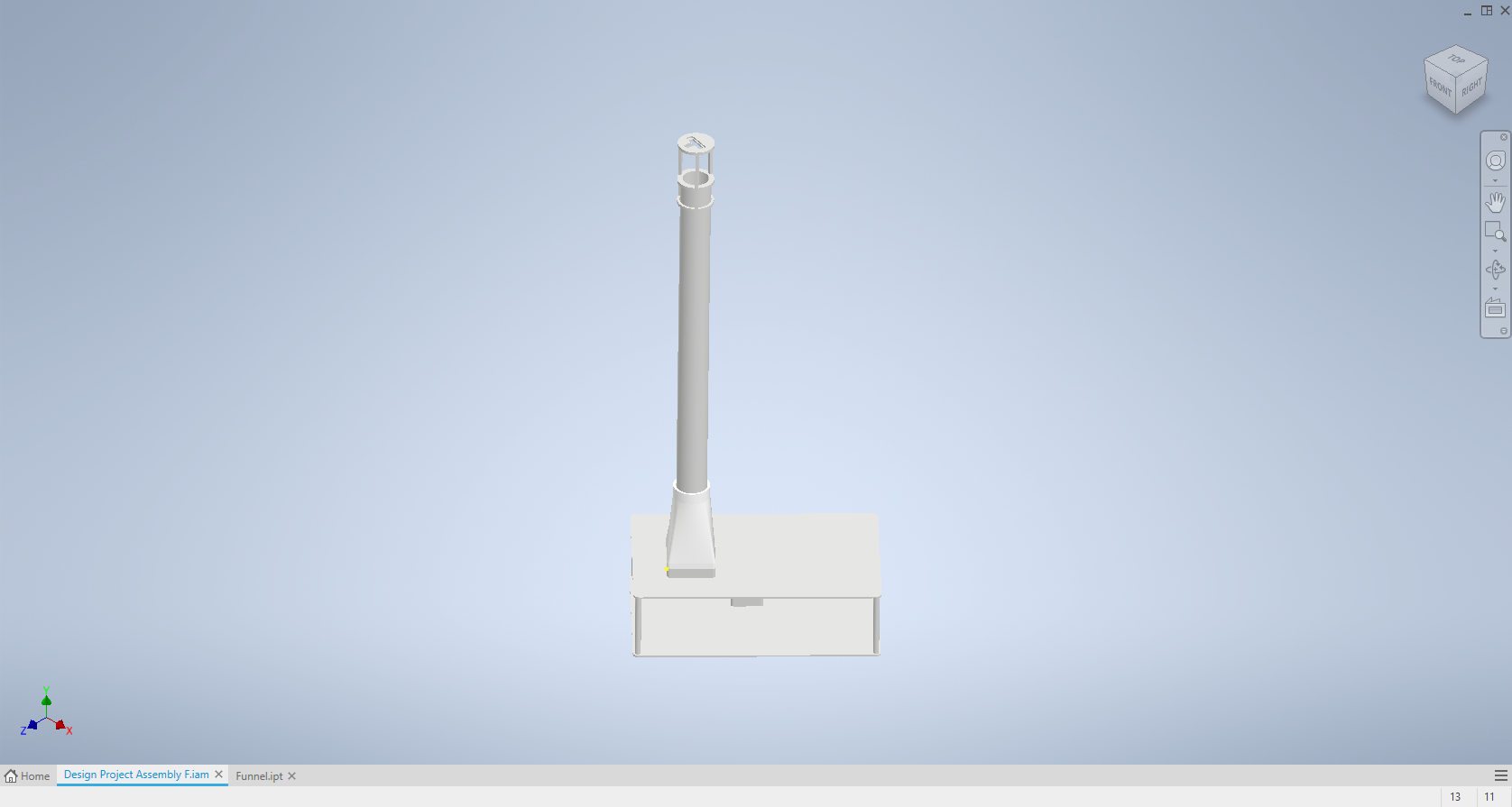
This section documents models for all 3-D printed hardware parts and their iterations so far in the project. Figure 11 depicts the ideal final build of this product, excluding electrical components, however the fixtures depict locations.
Figure 1. Funnel iteration one
Figure 2. Funnel iteration four
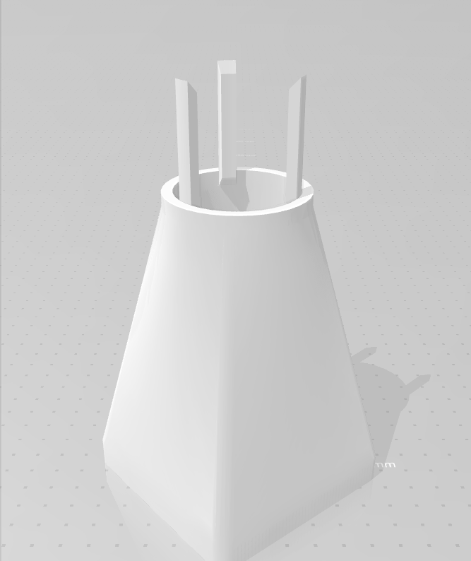
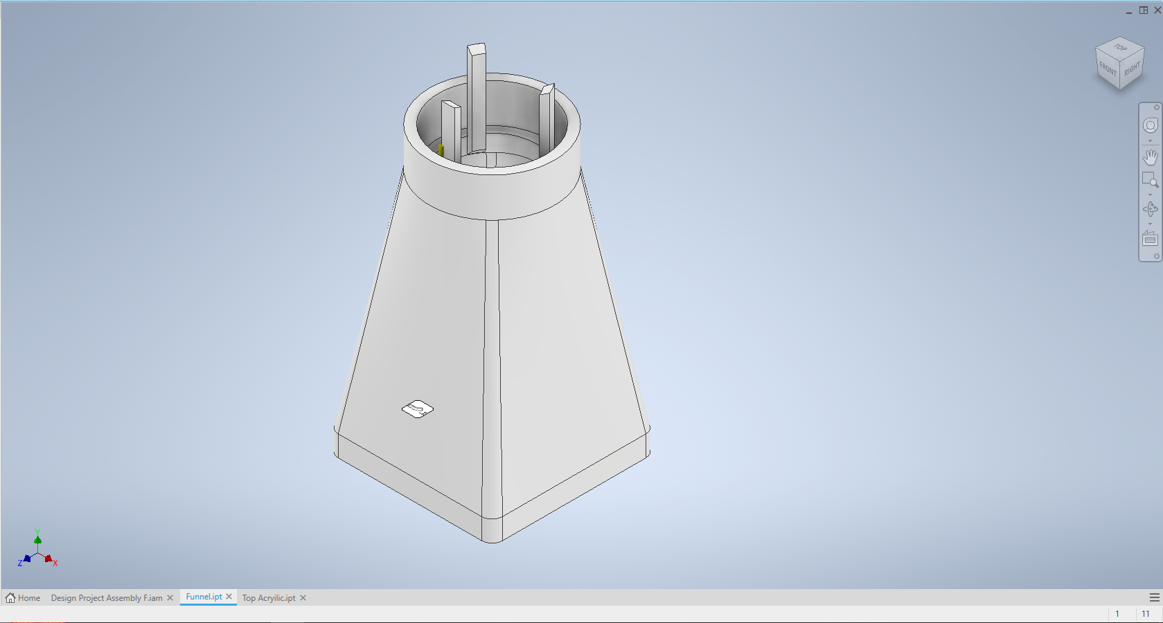
Figure 4: Funnel iteration five (Current)
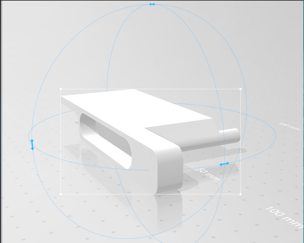
Figure 5. Servo motor flap. Design One
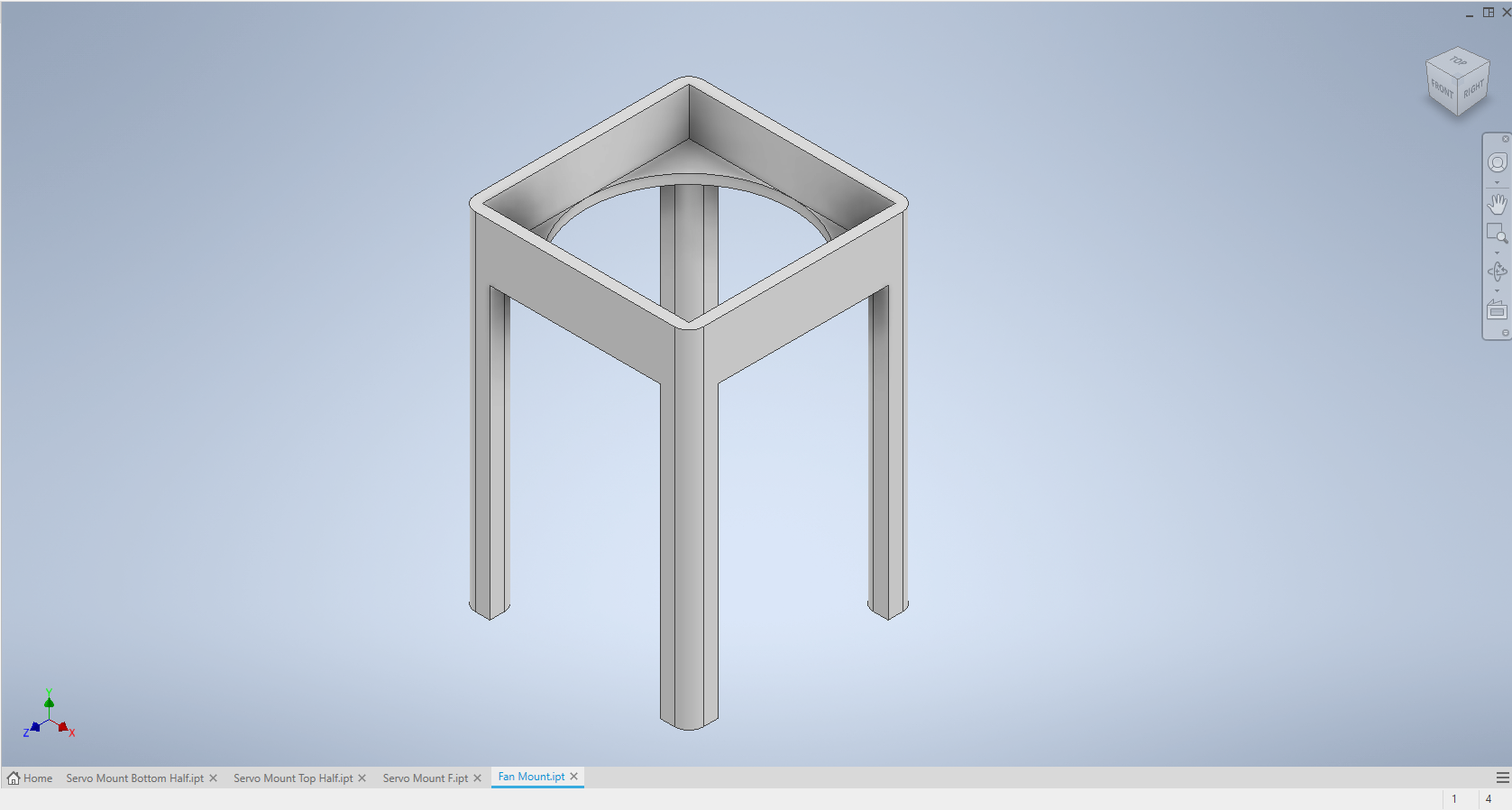
Figure 6. Fan mount and stand. Design one
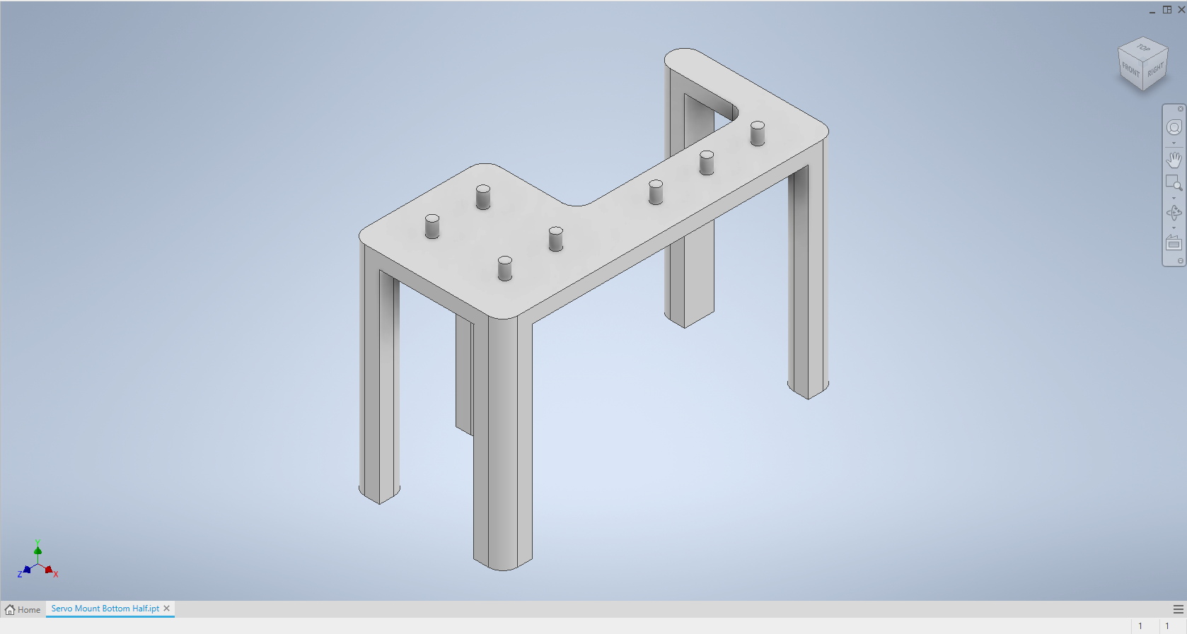
Figure 7. Servo motor stand. Design one
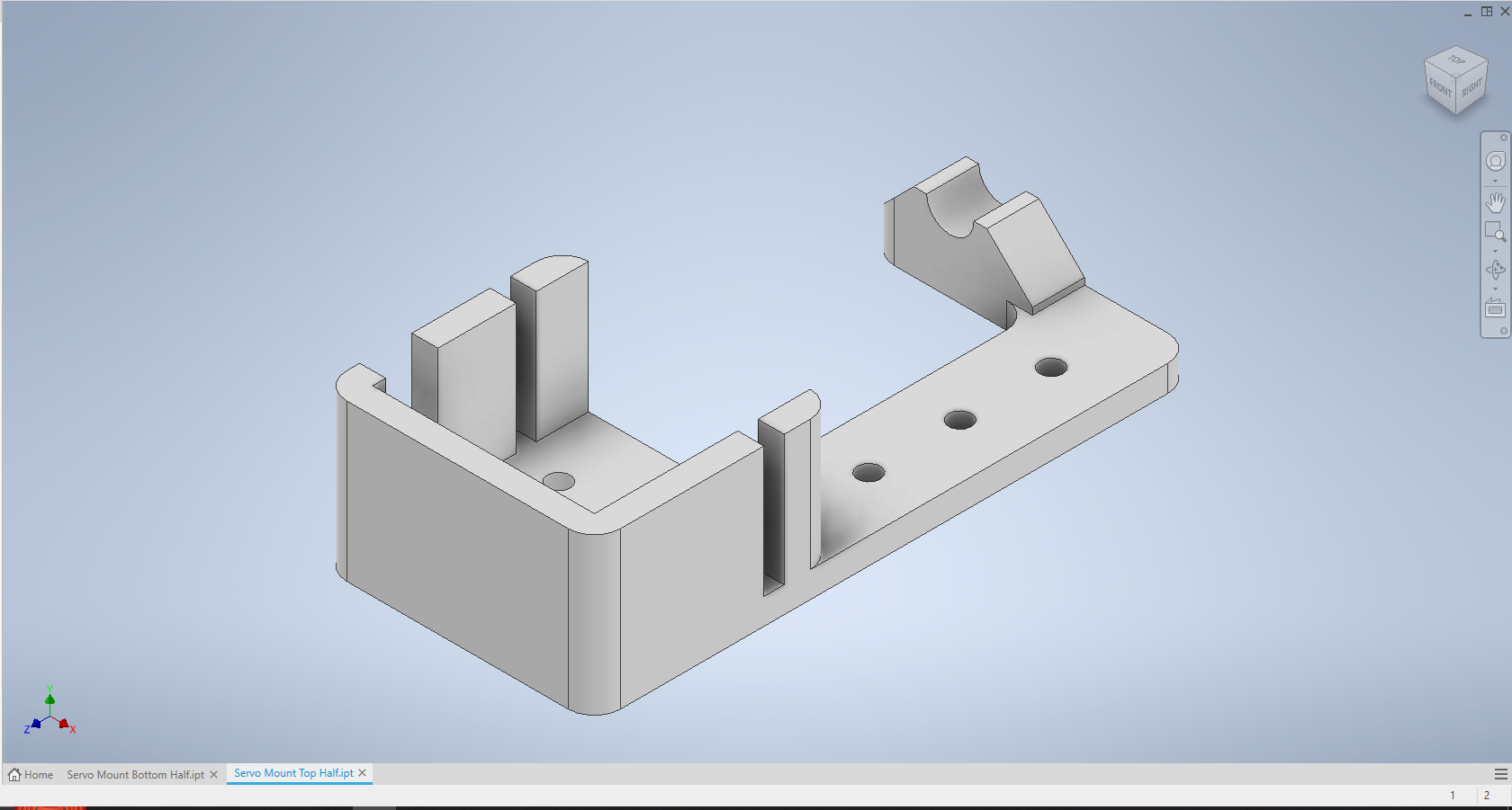
Figure 8. Motor mount. Design three
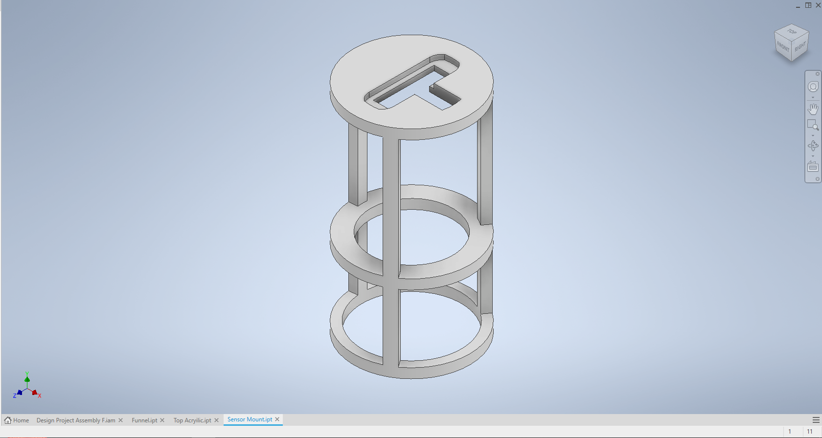
Figure 9: Sensor Mount Design 2
Figure 10. Current fixture testing setup/assembly
Figure 11. Ideal housing final design
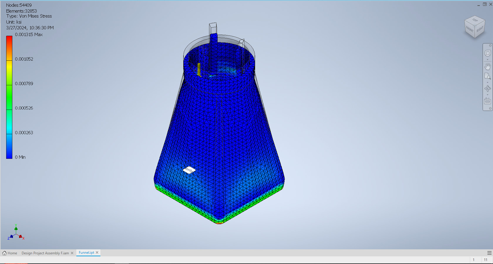
Figure 12. FEA simulation on the nozzle
To simulate some of the stresses on some of our most important prototype pieces an FEA analysis was done to determine if the modeled design was suitable and if there are any potential problems with our model. First, a force was applied to the top of our modeled funnel to simulate the force of gravity and the weight of the acrylic tube acting on it. Then a constraint was placed on the bottom of the model to simulate its contact with the acrylic sheet and fan housing. Then the simulation was performed.
Since the system identification process is currently in progress, our primary mode of engineering analysis was inspection during physical tests with essential hardware components.
The process followed is:
All hardware figures are referenced from the models and design section above.
Whilst planning the hardware setup for this project, the first component we decided to choose was the fan that provides the airflow to levitate the ball, and decided to build the rest of the hardware around this central component. The fan that was selected is an AMD computer CPU fan designed originally for the movement of cool air into a computer while it is in operation. The reason this fan was chosen is that group members had utilized a similar fan in similar applications for past projects, so it demonstrated promise for use in ours. Initial testing revealed that the fan not only had enough total airflow to propel a ball to the necessary height within a tube, but also had PWM control allowing users to adjust its speed, and therefore theoretically the airflow and the height of the ball.
The tube that was selected is a 24-inch long 1.75-inch diameter impact-resistant polycarbonate tube. These parameters were selected to one; best fit the ping pong ball without it touching the sides of the tube during operation, and two to provide enough height for variation in demonstrations while still maintaining the size parameters set by the initial project proposal. As for the material selection, polycarbonate was chosen as it allows users to observe the system while in use and is impact-resistant if the system were ever to be accidentally tipped over or dropped.
For the funnel that connects the fan to the tube, we went through several design iterations before finally creating one without present issues. These funnels were all designed using Autodesk Inventor and 3-D printed using PLA filament for rapid prototyping. Originally the funnel was a simple design seen in Figure 1, essentially a loft between the outside of the fan and the inside of the tube, but this design had a major oversight. When the tube was placed on top of the funnel it didn't contact the funnel on any flat surface which led to a tendency for it to be unstable and often tip over. For the next funnel iteration seen in Figure 2, this flaw was fixed by adding a horizontal ledge around the side of the funnel to the tube attached. This design had enough stability to test but did not lead to the airstream development the group had hoped for. The third version features a modification of the inside of the funnel by adding extra material which changed the interior shape of it into a cone instead of a square. Additionally, with this iteration, we shortened the bottom of the funnel around the fan to make room for a new test stand to increase the efficiency and ease of testing. This test stand is pictured in Figure 6. When testing this new funnel design we found that it performed worse for developing airflow, but we did discover a new issue when testing it too. Since the air in the funnel is going from a larger area at the fan to a larger area at the tube, a pressure difference is created at the funnel's opening that can result in the ball becoming trapped. For iteration 4 of the funnel seen in Figure 3, we sought to fix both of these problems with two design changes. The first is simply going back to the square interior for the funnel to improve the airflow development. To solve the pressure difference issue, we changed the cylindrical insert at the top of the funnel that goes into the tube with three prong-like structures. With the cylinder gone the airflow into the tube was improved, and the prongs prevented the ball from getting stuck. The final funnel design in Figure 4 was created after the previous one broke during testing. It added a ring of material outside where the tube sits to help secure the tube and prevent it from falling over.
Once the basic prototype of the fan, funnel, tube, and stand was created we began early testing. Quickly we discovered a few issues with the physics of what we had built so far. Firstly is the way the fan itself functions. When given a PWM signal voltage of zero, the fan still produces at least some airflow. Although this is not enough airflow to lift the ball, it still can slow its descent in the tube. Even if the fan is shut off completely the fan continues to spin due to inertia creating some amount of airflow slowing the ball's descent. To solve this issue, a small 3-D printed device with a servo motor-mounted flap was created. The base mount and flap for this assembly are shown in Figure 7, Figure 8, and Figure 5 respectively. This sits next to the fan's location and uses the servo to adjust the airflow that reaches the fan, as shown in Figure 10. With this device, the fan can be on full power at all times while the airflow is adjusted with the servo motor instead. This allows for more precise adjustments of the airflow and for the ability to stop all airflow almost instantaneously.
Originally for the sensor, we chose an ultrasonic sensor for determining the ball position. In testing, however, it was discovered that the tube interfered with the ultrasonic sensors functionality rendering the data received unusable. This is most likely due to the ultrasonic waves colliding with the sides of the tube and creating data that is not based on the ball itself, which in the current setup is almost impossible to work around. Because of this, we switched to an IR sensor with the hopes the sensor would perform better in the current environment. This sensor is currently still being tested and shows potential for use in the final product. The mounting for this IR sensor that sits on top of the tube is shown in Figure 9.
For the overall assembly, it was decided that since the priority of the project is educational use, the way the system is housed should lend itself to the educational use of the system as well. Because of this, we decided the housing should allow users to visually see all necessary components at all times to help them gain a better understanding of what the system is doing. The housing that was ultimately decided on is made simply by connecting two acrylic plates at the corners with metal standoffs. Then all components are connected to either the top or bottom plate, and the top plate has cutouts for certain components such as the potentiometer knobs and polycarbonate tube. Although we have yet to put together this complete housing assembly, a drawing of it is seen in Figure 11 above.
Initially, we were trying to get a step response using an open loop model, but we realized that for any given fan speed and motor angle combination, the system was unstable since leaving the system at any configuration led to the ping pong ball either sinking to the bottom of the tube or shooting up to the top. Our suspicions were confirmed when we reviewed a paper [6]. We therefore decided to develop a proportional controller and analyze the system in a closed loop. A controller was implemented in Arduino IDE, and we tuned its gain through trial and error.
The system was then tested, and it displayed the expected results. The controller was functional, but the system experienced significant drift and overshoot, which of course, could be corrected with integral and derivative control. Similar experiments with IR sensors [6] have revealed that the sensor showcases different behavior at different obstacle distances. We now plan to identify the system response to different ping pong ball heights by collecting a dataset of sensor readings vs ball height.
The brain of the system was chosen to be an Arduino and the reasoning behind its selection is discussed in the hardware section above. Therefore, using the programming software provided by Arduino was a simple choice, as it provides a free, rapidly adaptable, and simple way to write and upload code to the Arduino.
Using the Arduino IDE any code can be uploaded to the Arduino and run indefinitely as long as the system is powered.
The Arduino more or less handles everything for general system operation this includes running the sensors, fan, servo motor, and of course, the control algorithm that loops many of the subsystems together. We will be using a PID algorithm to maintain control of a ping-pong ball. The use of a PID controller was predetermined due to the product specifications given, but its versatility, simplicity, and accuracy make it the best choice regardless.
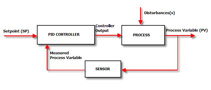
For our system, the control algorithm works as follows, the Arduino acts as the brain of the system and everything in the ‘control loop’, see Figure 12 [3], runs through it.
Figure 13. Basic closed loop control block diagram
a. PID Controller → Arduino
b. Process → Servo & ping pong ball system
c. Sensor → IR Sensor
The user inputs a desired height into the system, the setpoint, and that reference is constantly fed to the controller until it is changed. Meanwhile, the sensor observes the ball's position and feeds that into the controller as well. Here the controller calculates the error, the difference between the setpoint and the actual position, and uses the error to calculate the appropriate response to the actuator. In any case, a properly functioning controller should bring the process variable, ball position, closer to the reference, and depending on your performance requirements it can do this in several ways (aggressively, slowly, with/without overshoot, and so on). A PID controller calculates the adequate response by taking the current error, multiplying it by a constant gain term, and summing them up, as shown in equation (1) [4].
 (1)
(1)
Where P, I, and D are the proportional, integral, and derivative terms,  ,
,  , and
, and  are the respective gain terms, and
  is the error.
Each part of the controller has a different effect on response. From equation (1) you can see that the ‘P’ term or ‘proportional’ term is just the error multiplied by some constant value, so a higher proportional gain will give a faster, more aggressive response. In most cases just a ‘P’ controller is not enough, so we add the other terms to account for past and future error. The ‘I’ term or ‘integral’ accounts for the ‘history’ of the error signal, and will weigh the output signal higher or lower depending on how long there has been error. Finally, the ‘D’ term or ‘derivative’ term helps predict future error by taking the time derivative of the previous current and previous error values. This has the effect of protecting the system from sharp fluctuations and preventing large overshoots [4]. This is a simplified explanation of these terms but in general, by adjusting the gains of each you can vary the response of the system, to the same command!
With this understanding, it is now possible to talk about the advantages and disadvantages of using PID control for this project.
Advantages
Disadvantages
While the bulk of the Arduino code is for the PID control algorithm the system code also watches for user input and adjusts operations based on changes to them. Basic inputs (setpoint, controller gains, sampling rate) can be changed in real-time, albeit roughly, via dials, but if a user requires fine-tuned values they can input directly into the IDE or through a Matlab UI, discussed next.
Please reference Appendix B for the code we are currently using. The major features of this code are the servo and sensor libraries and the controller code. Arduino has built-in libraries that make working with hardware straightforward. The controller code is currently set up as a PI controller. System identification will be done with a P controller, but the ‘Integral’ portion was a quick addition and served as validation. With the integrator installed steady state error was effectively eliminated, however the sensor still outputs random bursts of noise which disrupts the balls steady position.
The Arduino/Arduino IDE handles running the demo’s general function as described in Sections 6.3.1 and 6.3.2. While this runs our system from an operational level, the other ‘half’ of this project is its educational capabilities. To cover educational requirements a GUI, live data plotters, model simulators, and more is necessary.
The Arduino IDE does have some data visualization capabilities but it is quite limited. Customization is limited, the x and y axes automatically adjust to data (which has the effect of visually skewing data), and the plotting UI is limited strictly to plotting. This last point is especially important since the GUI will be critical for this product. Users should be able to see system data live, simulate mathematical models for experimental comparison, and easily change operating parameters (tuning control gains, adjusting sampling rates, changing the ball’s setpoint). The Arduino IDE simply does not have the capability for this.
Matlab however, has all of these capabilities packaged into its GUI app designer. With the app designer, you can have live data plotting, fields for user inputs, and toolboxes with functions built in for simulations. Matlab also has a toolbox that can allow for capability between Arduino and Matlab. This handshaking allows the data on the Arduino to be bussed across a PC’s serial port where it can be taken live by Matlab. This interaction goes both ways and Matlab can also send information to the Arduino (i.e. input changes).
The result of our hardware testing with the proportional controller was as follows:
The result of our FEA was as follows:
Engineering standards play a crucial role in the design process of any project. This project does not require us to strictly adhere to any standards but understanding the relevance and applicability of them can help ensure a well-designed and reliable system. Below are standards that act as guideposts for the product:
Standards
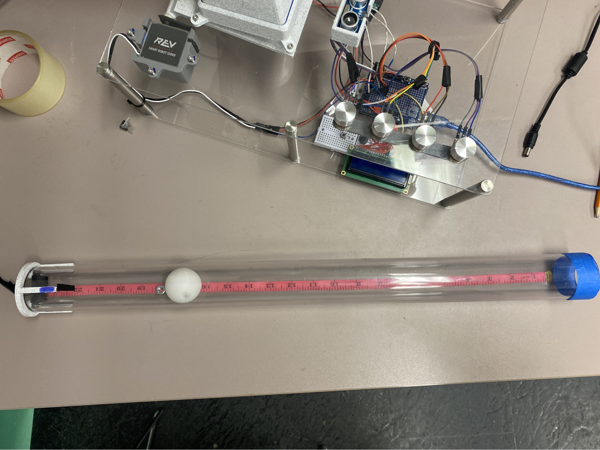
For the implementation of the final version of this project, we started by designing and fabricating the main acrylic plates; the rest of the project is mounted in and around them. These plates were designed in AutoCAD and created using a laser cutter. The overall size and design were selected based on the previous hardware prototypes that had already been made for preliminary testing. Once these sheets were created they were connected with aluminum standoffs that held up each sheet at different heights. For the various hardware needed to house and use the motor and fan, the parts were modeled in AUTODESK Inventor and then 3D printed with PLA plastic. These parts were designed with screw holes in order to be attached to the acrylic. To attach the housing and mounting pieces to the acrylic holes located where the hardware was planned to be were drilled through the top plate to allow bolts to fasten the mounting to the bottom of the top plate and the fan housing to the top. The hardware on the bottom was designed to house a servo motor, which is attached to a flap, while the housing on the top simply houses the fan and allows for the funnel to be securely inserted. To properly secure the potentiameters to the top plate all four potentiameters were glued to a 3D printed PLA bar to hold them together. Then electrical tape was wrapped around the threaded portion of the potentiameters to act as a gasket. These were then inserted firmly into the pre cut holes from the bottom, and had aluminum knobs attached to the turnable portion of the potentiameters to act as an anchor. Finally, the tube assembly was created by having a IR sensor mount that is glued to the top of the polycarbonate tube, as well as a funnel attached to the bottom. Both the funnel and the mount were designed in Inventor and printed with PLA plastic. Once the funnel and mount were secured on the sides of the tube, the bottom portion of the funnel can be placed into the fan housing on the top plate of acrylic.
This section documents the implementation of the various hardware components of our system. Each section will cover the corresponding component's purpose, the basic operation, and the methods used to implement them.
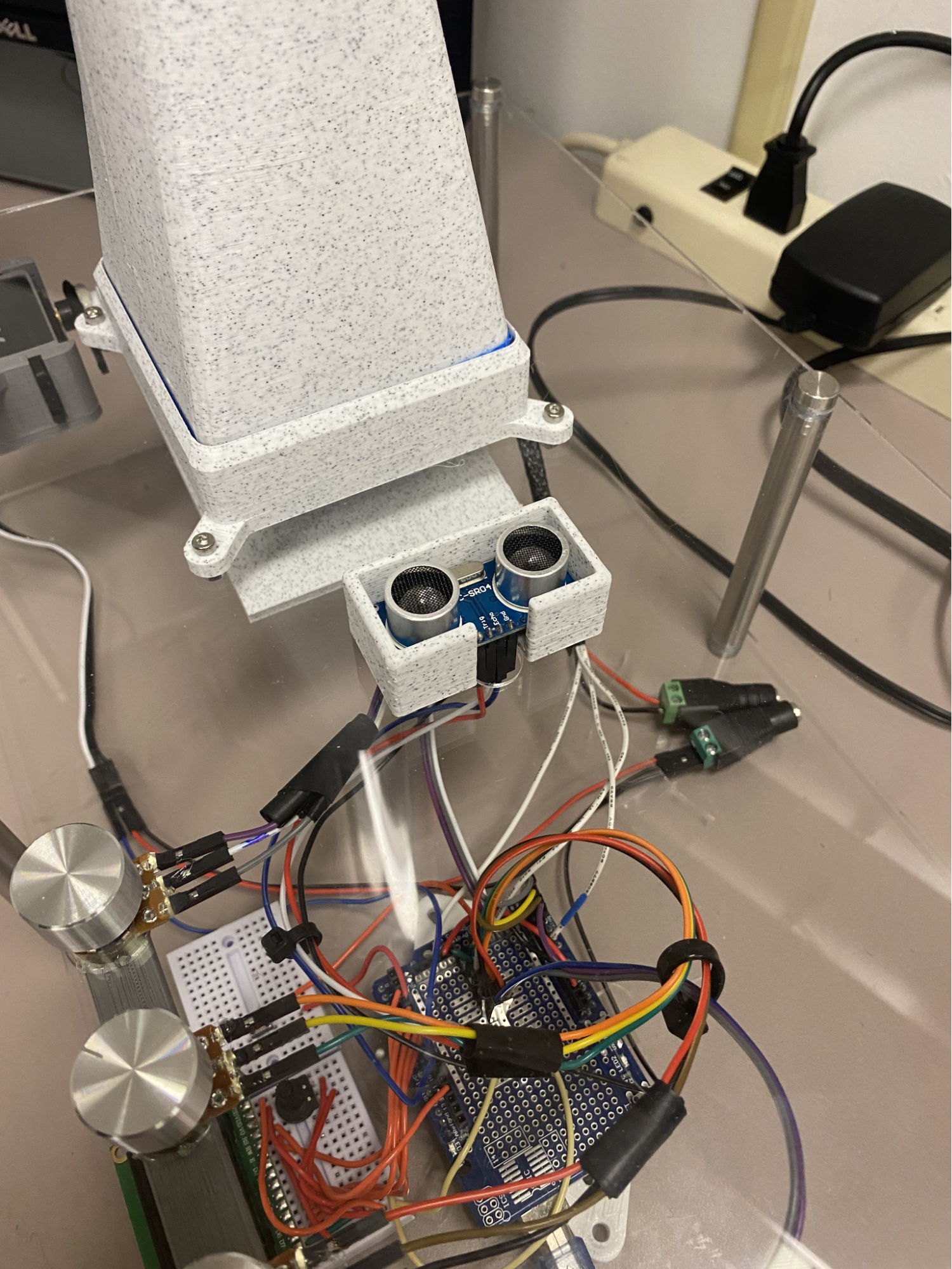
The infrared (IR) sensor is from Sharp and is the GP2Y0A21YK0F model, see Figure 14. This sensor's purpose is to observe the position of the ping-pong ball and feed the position data to the Arduino at the set sampling rate. The sensor is mounted to the top of the tube using a custom-made 3D-printed housing.
Figure 14. Mounted IR Sensor for ball position monitoring
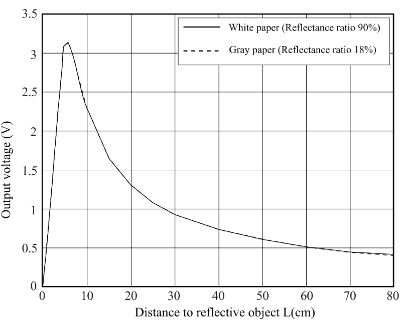
Each sensor has a calibration curve that looks like the one shown below, Figure 15 [1].
Figure 15. Sharp GP2Y0A21YK0F general calibration curve
This plot shows that the calibration curve is nonlinear and has a minimum operating distance of around 10 cm. Initially, we used a prepackaged Arduino library to run the IR sensor but the readings were inaccurate. We believe because the sensor is mounted inside a tube the typical curve was skewed. To get around this a manually calibration was performed by recording the sensor's voltage output at various locations in the tube and doing a linear regression to find the best fit equation. The calibration process is further discussed in the validation section.
The ultrasonic sensor is the HC-S404 model which comes in the Arduino starter kits. The purpose of this sensor is to act as an observer of a user's hand for reference tracking. With the ultrasonic sensor mode toggled on, the setpoint is determined by the user's hand and the controller will move the ball to your hand anywhere within the operating range. This sensor did not have the troubles encountered with the IR sensor, and the Arduino’s prepackaged ultrasonic sensor library was used to operate it. It is located on the top plate of the project, and is seated in a custom made 3D printed mount, Figure 16.
Figure 16. Implementation of the ultrasonic sensor for reference tracking
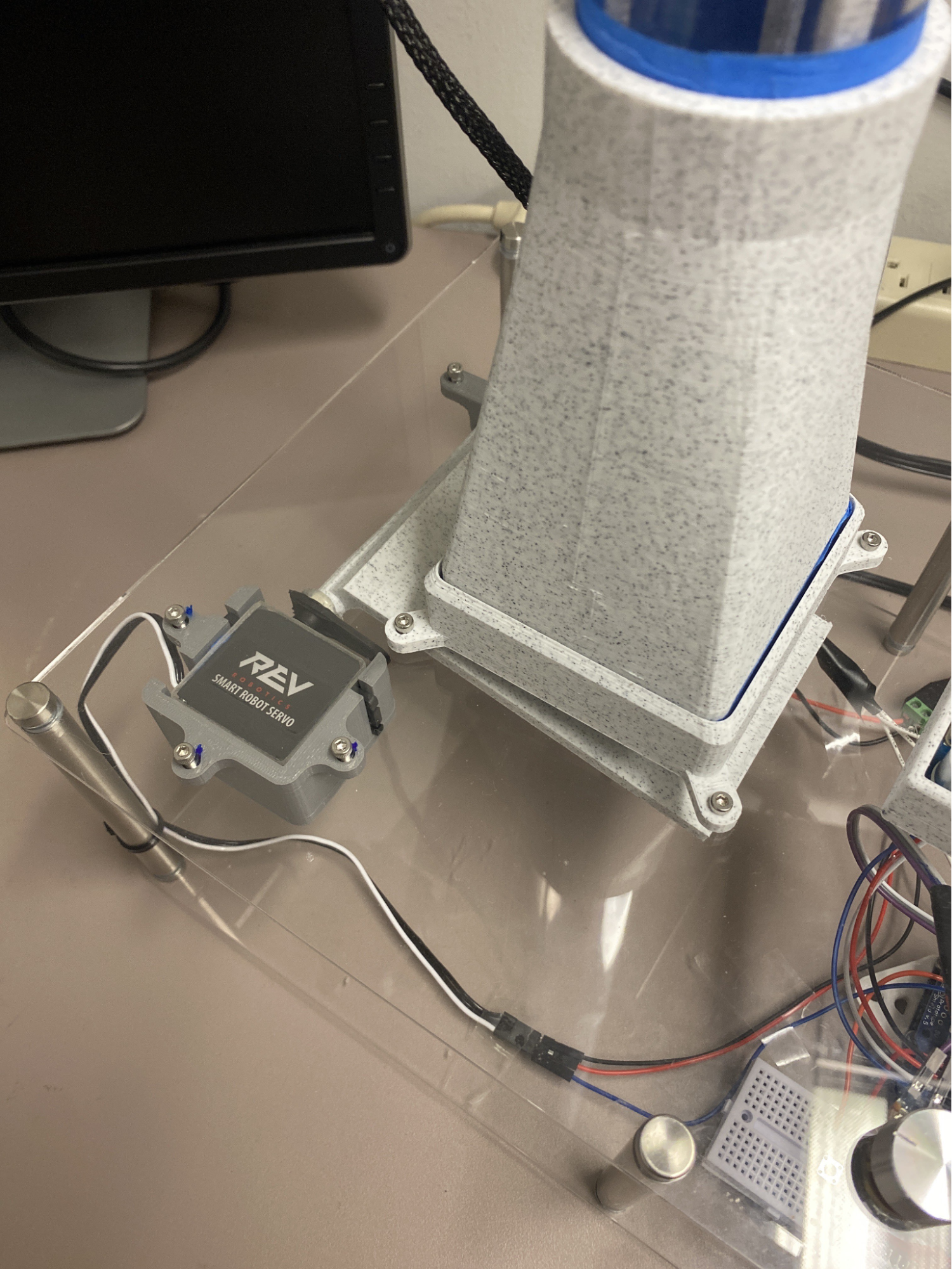
The servo motor used is a Rev-41-1097 servo motor from REV robotics. This motor was given to us by the project sponsor for use in the project. In the assembly this servo motor was placed within its own 3D printed housing which was secured with screws to the bottom of the top plate of acrylic, where it was hot glued to the 3D printed flap to act as an airflow regulator, Figure 17. The motor's angle bounds were set, and the motor was zeroed using the arduino IDE software. During operation the motor's angle is set by the onboard arduino depending on what the controller commands. To power the motor a 6 volt power supply is connected to a socket on the back of the assembly.
Figure 17. Implementation of the servomotor-flap system. Mounted beneath the funnel to control airflow to the tube, thus controlling the ball
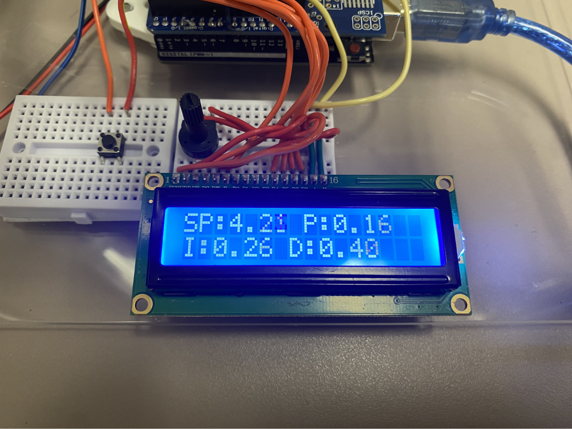
The LCD screen came prepackaged with the Arduino starter kits. The LCD screen outputs the parameters that can be adjusted by our potentiometers, the setpoint, proportional gain, integral gain, and derivative gain. This lets the user see the adjustments they are making in live time, without an external UI. The LCD sits on its own breadboard which has cables bussed to the necessary Arduino digital, power, and ground pins. See Figure 18.
Figure 18. Functioning LCD located on the lower base plate. Outputs setpoint, and three controller gains. Notice the neatly kept wires. Also of note is the mode switching button located to the left.
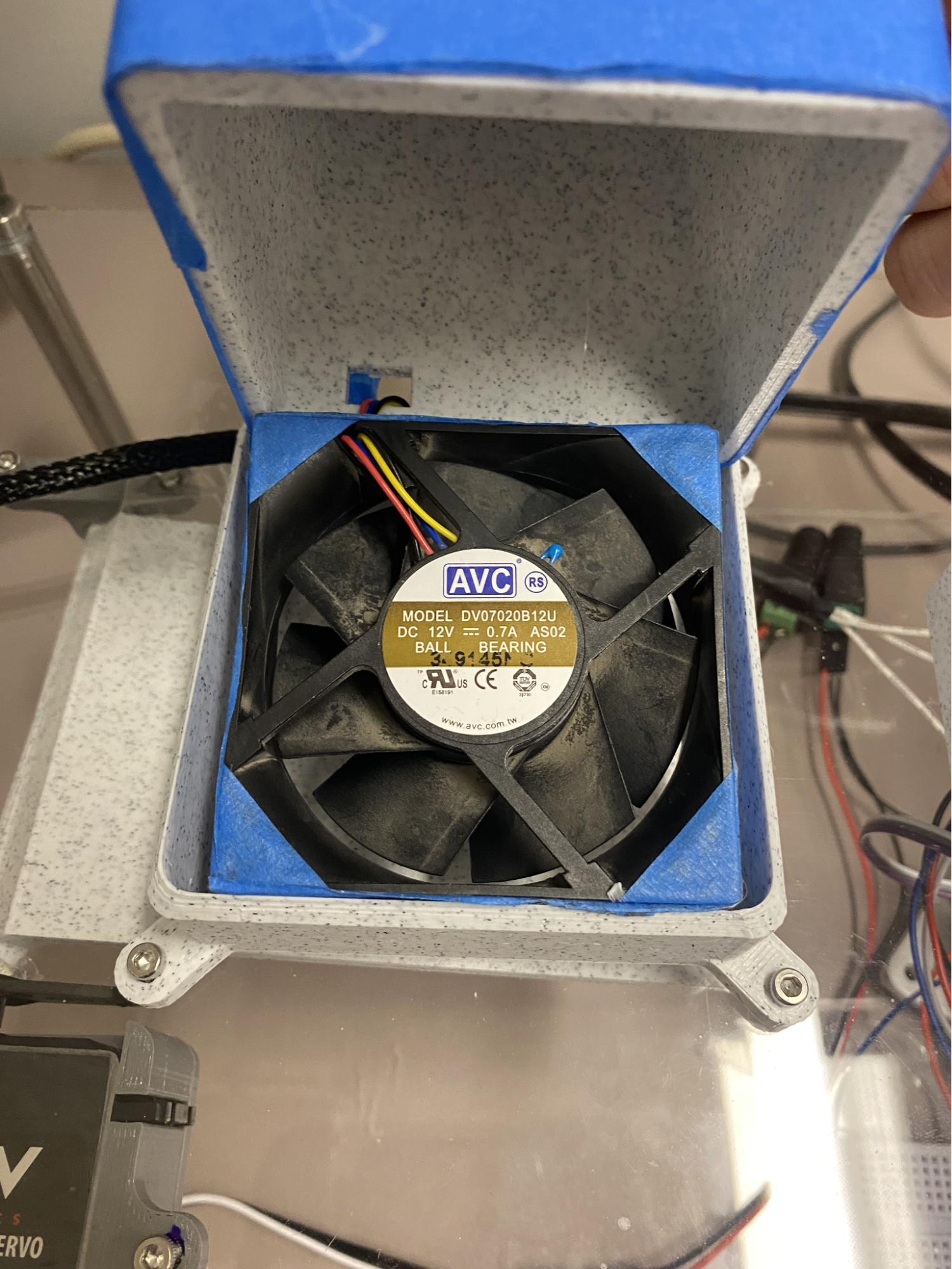
The ball is levitated by a 12 V computer fan, which spins at a constant rate, the max speed at full power. The computer fan sits inside of the nozzle directly underneath the ball. The wires are fed outside of the funnel and powered by a 12 V external power supply which sits in the back of the housing. See Figure 19.
Figure 19. 12V DC computer fan inside of the fan mount-funnel fixture. Wires are fed outward to the power supply.
Initially, the plan was to vary the speed of the fan as the systems actuator but due to slow response times and poor controllability the servo-motor flap system was chosen instead.
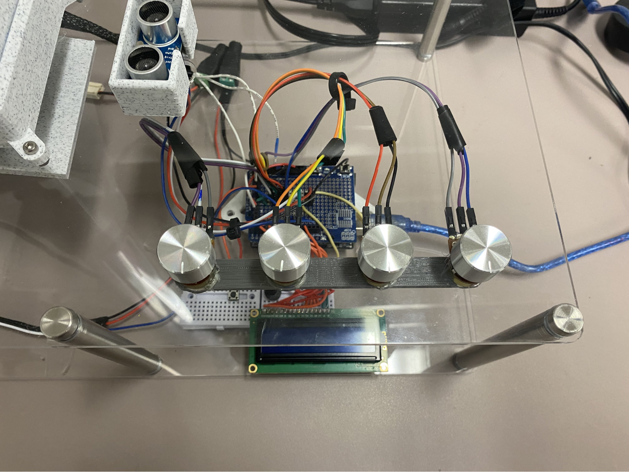
The potentiometers or control knobs are the interface for the critical parameters of the system. In the manual mode, the setpoint can be adjusted using the left most knob, and the controller gains, P, I, and D can be adjusted using the other knobs in either mode. See Figure 20.
Each potentiometer is bounded by reasonable values, 0 - 18 inches for the ball setpoint, and 0 - 2 for each controller gain, and has an increment of,  . Each potentiometer is powered by the Arduino and the sense cable of the potentiometers runs into an analog pin on the Uno.
Figure 20. Potentiometers for parameter control implemented on the top plate for easy access. From left to right is the setpoint, proportional gain, integral gain, and derivative gain control knobs.
An Arduino Uno is the microcontroller for this project. The Arduino acts as the brain of the system and handles all of the data, computations, sensor readings, and control output. The code run by the Arduino will be discussed further in Section 9.3. The Arduino has a prototyping board attached to it, which helps create more space for wires. All components that require 5 V power and ground are soldered to a common line on the prototype board. The cables were run neatly, and kept short when possible to help with student visualization of the signal and energy flows. Furthermore, the Arduino IDE is capable of live plotting of data that is bussed to the serial monitor, which is an extremely helpful tool for student visualization. See Figure 21.
Figure 21. Implementation of an Arduino UNO, the brain of the brain of the system. Notice the attached protoboard used to centralize the ground and power connections, as well as neatly organize the sensor pins.
Go to Appendix B for the full Arduino code.
The software being run on the Arduino can be broken into a few major sections. The declaration of variables (contains important constants that can be adjusted), the short functions used in the main body, and finally the main body, which contains the IR sensor code, its filters, the mode selection code, and the controller code.
In the beginning of the code, all the relevant libraries are called, and many variables are declared. The code uses the built in servo motor and LCD libraries. Here, the sampling rate and filter strength can be modified if necessary.
The ‘killSpikes’ function is the first filter applied to the IR sensor. This function takes 8 samples from the sensor, removes the highest and lowest values, and returns the average which is returned and used in the main body. This helps remove outliers from the IR sensor reading, which was a big problem since it disrupted the system's ability to settle. At times it recorded spikes that would correspond to a 4 inch disturbance in the ball's position, which was not happening in reality.
The ‘ultrasonic’ function is what runs the ultrasonic sensor for reference tracking. It sends a pulse of sound out, and uses the time delay of the return pulse to calculate distance. The function returns the setpoint, which is the distance recorded and a couple of offset values to account for the IR sensor's top down orientation, and the length of the ultrasonic sensor below the funnel.
The entire main body of the code runs inside an ‘if’ statement that only executes at the sampling period. Simply, if the sampling rate is 30 Hz, the main body will execute 30 times a second.
The first thing the code does is calculate the position of the ball by taking the filtered voltage from the ‘killSpikes’ function and then is run through a software lowpass filter to further smooth the signal. The fully filtered signal is then put through the regression function from Figure X. Next the mode selection code is run, which is just a series of ‘if’ statements that depends on the previous button press. One ‘if’ block uses the manual mode setpoint selection and the other uses the ultrasonic sensor reading. Then the controller gains are declared using the other three dials.
The next major section is the control output calculation using the PID algorithm. First the error is calculated, simply the difference between the IR sensor reading and the reference. Then the error is run through three ‘branches’ of the controller. The proportional branch is just the error multiplied by the proportional gain. The integral branch is the integration of the error signal multiplied by the integral gain. Rectangular integration is used here, with the reference being 0 error. Finally, the derivative of the error signal is taken between every timestep, which gives the rate the error signal is changing. That value is multiplied by the derivative gain to yield the derivative branch value. All three components are summed up, giving the ‘abstract’ control output. The control output is constrained and mapped to a servo motor angle, thus giving the real output value. This code repeats continuously, updating the output at the sample rate set by the user.
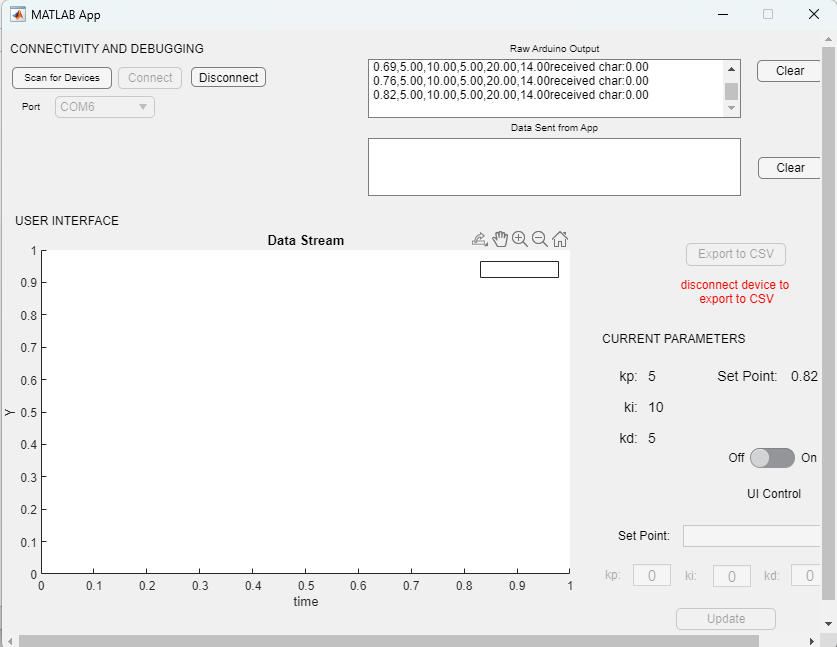
In order to implement more sophisticated control tools in the future, we set up a MATLAB application to connect to an Arduino and plot and monitor its data. The app allows the user to quickly plug in the Arduino into their device and access the plethora of analysis tools that MATLAB offers. The app supports bi-directional communication, although the App to arduino communication needs further optimization.
In the future, we believe that the application will be very helpful for closed loop system identification, which would bolster the educational potential of our product, and help figure out optimal PID gains.
Figure 22: MATLAB App UI
Currently, the app supports live Arduino output plotting and even allows the user to export the data to a CSV file. However, only limited number of high-level commands are able to be sent to the Arduino. The app to arduino data stream needs to be fixed.
Since this system is meant to be used in educational settings, one of the goals of this project was to display the inner workings of the hardware for students to see. So, our team tried to space out the hardware components so that each individual component could be seen. To ensure durable connections, connections were soldered with the potentiometers, but to allow for customization, a breadboard was used as well.
To validate the functionality of this project, the group ran through multiple PID gains and reference heights to ensure the system continues to function as usual throughout. Functionality was determined by stability and accuracy.
During this testing it was noted that no matter how much the system was tuned there would always be some amount of oscillatory motion from the ping pong ball. It was theorized that this oscillatory motion was not inherent to the system, and that something must be wrong with the controller.After investigation of the code it was discovered that the data coming from the IR sensor was being over filtered. Any filtering will add delay to a signal and the first implementation of our filter was adding a delay of around 2 seconds to the real ball position and the generated sensor reading. Essentially, this meant the system was alway attempting to act upon a state that it was no longer in, leading to suboptimal responses. This was easily fixed by increasing the  term in the filters code to reduce how much the data was being filtered by. Ultimately, this led to better performance from the system all around.
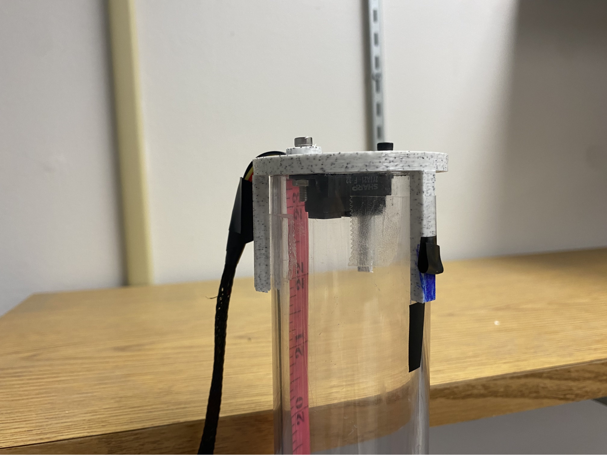
An additional issue that was discovered earlier in assembly and testing was inaccurate reading from the IR sensor, briefly discussed in section 9.2.1. When the IR sensor was originally implemented a prebuilt Arduino library which used the sensor voltage output to backout the balls distance. This library used a regression function characterized by the curve in Figure 22. The library worked well when measuring things outside of the tube, but once the sensor was mounted to the tube, the output data became noisy and inaccurate. It is believed the tube shifted the expected calibration maximum value to the right, drastically reducing our operating range. Some literature suggested using colored strips inside the tube to solve this problem but limited success was found with this. Our solution was to do our own calibration and use our own regression equation. To do this we measured the voltage at 0.5 inch intervals over the length of the tube, Figure X shows the calibration experiment setup.
Figure 23. IR sensor calibration setup
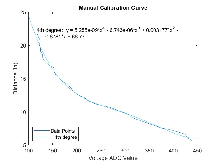
After recording the sensor output at the various lengths we plotted the points in Matlab and used the plotting functions built in fitting function to find the regression equation. A fourth order fit was chosen and the equation is shown below in Figure 23.
Figure 24. Calibration curve with regression equation
This helped significantly with the height readings, however there was still the noise issue that was fixed using the filtering methods addressed in Section 9.3. After filtering, the sensor was accurate with about 0.25 - 0.5 inches throughout most of the tube, with a few locations being nearly perfect. This accuracy was found to be more than adequate for this project.
When designing our project we achieved a product design almost entirely based on our original and approved revised plans for the project. Some of these completed portions of our design were the aesthetic and functionality of our PID control demo as well as the educational aspects. Due to the completion and adherence to our initial design, a score of 97 out of 100 would be an appropriate estimation of our implementation achievement. However, we were unable to complete some of our secondary goals for our project like a digital twin due to unforeseen complications during the system identification steps. To complete the core goals of our design we had to prioritize testing the system and getting the most accurate responses leaving us unable to complete our secondary goals like a digital model. However we did the legwork to prepare the system for this step so it can be more easily implemented in the future. Also, these were not goals initially assigned to us and were added after the fact upon customer discussion. To assess the functionality of our product we have to consider the success of our tests and how well our product performs. When rating the system out of 100 a score of 95 would be an appropriate score for our product due to the successful usability of our project and the accuracy of our systems. One reason for our testing being 95 instead of 100 is due to the complexity of finding a 100% accurate mathematical model for our open loop system. An additional unforeseen complication was the difficulty of testing our system leaving us with minimal time to work on other portions of our project.
Overall, this project has led to the creation of a well put together PID control demo that can be used for effective educational purposes in a classroom environment. This demo successfully conveys the ideas and concepts of a PID control system in way that is easy to visualize and interact with. The system is fully functional, allowing the user to set the setpoint to all valid positions within the tube, and each PID gain can be set individually to see the reaction and effect on the system. The primary findings of the project were, as we initially expected, that a well designed visual system does allow students to better understand the concepts of a PID control system. When shown off, the system had large amounts of engagement with students and allowed for the concepts to be explained in an understandable manner. Ultimately, this project has aligned with the goals set out at the beginning.
We believe that the product we delivered to our sponsor was a more than adequate system. It covered almost everything we laid out in our product design specifications from the initial design. However, a couple of things we did not fully integrate, some things to improve, and some future work that should be completed.
First the things we did not add. While all of these are minor and do not affect the operation or functionality of our product, they would improve the quality of the product.
A built in power supply was an original customer request, but after conversations with Dr. Estes it was determined that powering the system with wall power was sufficient. It would make the system more portable if it was powered by its own means with a battery, but it is hard to imagine a situation where the system will be used without an available laptop for the Arduino or outlets for the fan and servo motor. At the very least an in house 5V supply should be considered for the Arduino to be powered without external help.
This was requested in the original specifications by the customer, but unfortunately it slipped through the cracks. We implemented four other knob adjustable settings, but by the time we realized we forgot the sampling rate adjuster it was too late. It’s a really simple addition, just another potentiometer added alongside the others. For now, the sampling rate can be easily changed in the code. Of course everything can be improved but here is a list of most important improvements.
The current mount is not fixed in place very well and unfortunately the orientation of the sensor is critical to the calibration. If it is rotated out of the position that it was calibrated in, then the calibration is no longer valid. Currently we have it ‘keyed’ using a sharpie mark on a leg of the mount and the tube. This way if the sensor does move it can be put back into place. We wanted to improve the mounting for the sensor to make it more permanent but did not want to have to redo the calibration so it was left as is.
As discussed in Section 9.3, the PID controller output is constrained and then mapped to a corresponding angle. Currently the mapping assumes a controller output range of -12 to 12 and that is related to a 123 to 85 degree angle. The angle bounds correspond to the physical limits of the motor within the housing. So the angle bounds are more or less fixed (at least magnitude of the difference between the two angles, the starting and ending reference angle can be anything and depends on the zeroing of the motor).
However, the selected error range is something to be investigated, and possibly improved upon. This error range was initially chosen assuming a 24 inch tube, and a setpoint of 12 inches. If you are running only a P controller with the gain set to one, the range of error is in fact -12 to 12.
The first problem is more simple, the actual operating range of the sensor is not 24 inches. We are losing about 4.5 inches from the top due to the minimum operating range of the IR sensor, and about 2 inches from the bottom due to the resting point of the ball. So, the simple solution is to adjust the ideal range to accommodate these losses. The second problem is more complicated. Still assuming a simple proportional controller, just by changing the P gain, you reduce the error range. For example, if P is set to 0.5 the possible error range is reduced to -6 to 6. This reduces controllability. To expand on this, adding the integral and derivative control terms makes the error range unbounded. The integral term can grow indefinitely if the error does not change, and depending on the rate the ball comes into the setpoint the derivative term could be very large. Again the magnitude of those terms also depends on the I and D gain. Due to this, we believe the error range should be more robust, or the ‘map’ function abandoned altogether and replaced with something better. We tried making a more robust error range, one that accounted for the gains and integral/derivative terms but it did not work. For now, the -12 to 12 range works so it is not overly critical, but we believe some other alternative should be investigated.
Finally, something that we would like to add to greatly increase the quality of our product.
This semester, Dr. Estes suggested to us that we attempt to do system identification on the system in order to get a mathematical model of our system that can be used to help further the educational benefits of the product. We were close to finishing this effort, and Dr. Estes helped us get a rough model of our system. However due to difficulties and setbacks with the system ID we did not get to validate the model. This is something that should be pursued and could be greatly useful for engineering students taking his digital controls course.
For this effort, some things to note are that the system is unstable in open loop meaning closed loop system identification is necessary. Dr. Estes has a Matlab script that can help make this process easier, and has been a useful tool for us. Furthermore, any modifications made to the system will invalidate a model so it is important to have a full built system before starting system identification. The delay faced with system identification was due to our hesitancy to build a permanent system. Once we finalized things it made subsequent work much easier.
References
ARDUINO CODE:
#include <Servo.h>
#include <LiquidCrystal.h> // includes the LiquidCrystal Library
LiquidCrystal lcd(12, 2, 4, 5, 6, 7); // Creates an LCD object. Parameters: (rs, enable, d4, d5, d6, d7)
Servo myservo;
float val;
float previousTime = 0;
float currentTime;
// CHANGING SAMPLE RATE
float samplingRate = 30.0;
//
float interval = 1 / samplingRate;
float integral = 0;
// FOR CHANGING THE FILTERING HIGHER = LESS DELAY
float omega_c = 15.0; // 15 works good
//
float y_km1 = 0;
float u_km1 = 0;
float error;
float dis;
int sensorpin = A0;
float servo_val;
float derivative;
float previousError = 0;
float disturbance;
float disturbanceMagnitude = 3.0;
float combined_servo_val;
const int trigPin = 8;
const int echoPin = 10;
int Spin = A5;
int Ppin = A4;
int Ipin = A3;
int Dpin = A2;
float setpoint;
float required_height;
volatile int lastDebounceTime = 0;
volatile int debounceDelay = 200;
volatile int MODE = 0; // Declare MODE as volatile for use in interrupt
void modeSwitch() {
if (millis() - lastDebounceTime > debounceDelay) {
MODE = (MODE + 1) % 2; // Toggle MODE between 0 and 1
lastDebounceTime = millis();
}
}
void setup() {
myservo.attach(9);
Serial.begin(250000); // Initialize serial communication
pinMode(A1, INPUT);
pinMode(trigPin, OUTPUT);
pinMode(echoPin, INPUT);
lcd.begin(16, 2); // Initializes the interface to the LCD screen, and specifies the dimensions (width and height) of the display
pinMode(3,INPUT_PULLUP);
attachInterrupt(digitalPinToInterrupt(3), modeSwitch, FALLING); // Attach interrupt to MODE switch
}
float killSpikes(int sensorpin) {
float loopcount = 8;
float sum = 0;
float x = 0;
float avg = 0;
float hi = 0;
float lo = 0;
hi = lo = analogRead(sensorpin);
for (float i = 0; i < loopcount; i++) {
x = analogRead(sensorpin);
sum = sum + x;
if (x > hi) hi = x;
if (x < lo) lo = x;
}
return avg = (sum - hi - lo) / (loopcount - 2);
}
float ultrasonic() {
float setpoint;
float duration;
float ultra_reading;
digitalWrite(trigPin, LOW);
delayMicroseconds(2);
digitalWrite(trigPin, HIGH);
delayMicroseconds(10);
digitalWrite(trigPin, LOW);
duration = pulseIn(echoPin, HIGH);
setpoint = ((duration * .0343) / 2)/2.54;
if (setpoint > 26){
setpoint = 5.2 + 22.75;
}
return setpoint = 5.2 + 22.75 - setpoint;
}
void loop() {
currentTime = millis();
if (currentTime - previousTime >= interval * 1000) {
float V = killSpikes(sensorpin);
float unfiltered_dis = (5.25505026384692e-9) * pow(V, 4) - (6.74300953054098e-6) * pow(V, 3) + (0.00317702324785188) * pow(V, 2) - 0.678134109169401 * V + 66.77;
float y_k = (1.0 - omega_c * interval) * y_km1 + omega_c * interval * u_km1;
y_km1 = y_k;
u_km1 = V;
dis = (5.25505026384692e-9) * pow(y_k, 4) - (6.74300953054098e-6) * pow(y_k, 3) + (0.00317702324785188) * pow(y_k, 2) - 0.678134109169401 * y_k + 66.77;
float height = 22.75 - dis; // 22.75 is the reference height from the tube ruler
if (digitalRead(3) == LOW) {
MODE = MODE + 1;
if (MODE == 2){
MODE = 0;
}
}
if (MODE == 0){
required_height = (analogRead(Spin) * 18.0/1023.0) - .8;
setpoint = 22.75 - required_height; // Somehow this makes the setpoint w.r.t the tube ruler
}
if (MODE == 1){
setpoint = ultrasonic() - .8;
required_height = 22.75 - setpoint ;
}
// IF YOU WANT TO HARDCODE GAINS USE THIS COMMENT OUT THE ANALOG READS BELOW TOO
//float P = .5;
//float I = .5;
//float D = .2;
float P = analogRead(Ppin) * 2.0/1023.0;
float I = analogRead(Ipin) * 2.0/1023.0;
float D = analogRead(Dpin) * 2.0/1023.0;
//
error = dis - setpoint;
integral += (error * interval);
if (integral >= 12/I){
integral = 12/I;
}
if (integral <= -12/I){
integral = -12/I;
}
derivative = (error - previousError) / interval;
val = P * error + I * integral + D * derivative;
previousError = error;
val = constrain(val, -12, 12);
float servo_val = map(val, -12, 12, 123, 85);
//disturbance = disturbanceMagnitude*random(-1000,1000)*1.0/1000.0;
//combined_servo_val = constrain(servo_val+disturbance, 90, 120);
//combined_servo_val = round(combined_servo_val);
//int servo_angle = combined_servo_val;
int servo_angle = servo_val;
myservo.write(servo_angle);
//Serial.println(required_height);
//Serial.println(P);
//Serial.println(I);
//Serial.println(D);
Serial.print(height);
Serial.print(",");
Serial.println(required_height);
lcd.setCursor(0,0);
lcd.print("SP:"); // Prints "Arduino" on the LCD
if (required_height < 0) {
lcd.print(0);
}
else{
lcd.print(required_height);
}
lcd.print(" P:");
lcd.print(P);
lcd.setCursor(0, 1); // Sets the location at which subsequent text written to the LCD will be displayed
lcd.print("I:");
lcd.print(I);
lcd.print(" D:");
lcd.print(D);
lcd.print(" ");
previousTime = currentTime;
}
}
MATLAB App code:
classdef matlab_app < matlab.apps.AppBase
% Properties that correspond to app components
properties (Access = public)
UIFigure matlab.ui.Figure
WarningLabel_2 matlab.ui.control.Label
ExporttoCSVButton matlab.ui.control.Button
setpointLabel matlab.ui.control.Label
setpointCurrent matlab.ui.control.Label
setpointLabel_2 matlab.ui.control.Label
dCurrent matlab.ui.control.Label
kdLabel_2 matlab.ui.control.Label
kiLabel_2 matlab.ui.control.Label
kdLabel matlab.ui.control.Label
kpLabel_2 matlab.ui.control.Label
kiLabel matlab.ui.control.Label
CURRENTPARAMETERSLabel matlab.ui.control.Label
kpLabel matlab.ui.control.Label
iCurrent matlab.ui.control.Label
pCurrent matlab.ui.control.Label
USERINTERFACELabel matlab.ui.control.Label
UIControlSwitch matlab.ui.control.Switch
UIControlSwitchLabel matlab.ui.control.Label
kdEditField matlab.ui.control.NumericEditField
kiEditField matlab.ui.control.NumericEditField
kpEditField matlab.ui.control.NumericEditField
ClearButton_2 matlab.ui.control.Button
ClearButton matlab.ui.control.Button
UpdateButton matlab.ui.control.Button
BallSetPointEditField matlab.ui.control.EditField
DataSentTextArea matlab.ui.control.TextArea
DataSentfromAppTextAreaLabel matlab.ui.control.Label
CONNECTIVITYANDDEBUGGINGLabel matlab.ui.control.Label
WarningLabel matlab.ui.control.Label
DisconnectButton matlab.ui.control.Button
ConnectButton matlab.ui.control.Button
RawArduinoOutputTextArea matlab.ui.control.TextArea
RawArduinoOutputLabel matlab.ui.control.Label
PortDropDown matlab.ui.control.DropDown
PortDropDownLabel matlab.ui.control.Label
ScanforDevicesButton matlab.ui.control.Button
UIAxes matlab.ui.control.UIAxes
end
properties (Access = public)
port_list % list of all serial devices
arduino_port
arduino
data_to_send
set_point
kp
ki
kd
sensor_height
model_height
startTime
time_array
dataplot1
dataplot2
dataplot3
SerialTimer
PlotTimer
app_control
% kp_max = 10; % to set the range and increment for the knob limits
% kp_min = 10;
% ki_max = 10;
% kd_max;
% kd_min;
%
% ki_inc;
%variables to send to arduino
end
methods (Access = public)
function readSerialData(app)
% check if we want to use app control
if app.UIControlSwitch.Enable == "On"
write(app.arduino, "1");
else
end
% Check if data is available
if app.arduino.NumBytesAvailable > 0
% Read data from serial port
data = readline(app.arduino);
floatArray = strsplit(data, ','); %split it
floatValues = str2double(floatArray);
updateParameters(app,floatValues);
% get sensor height and model height
% Update textbox value
app.RawArduinoOutputTextArea.Value = [app.RawArduinoOutputTextArea.Value', data];
scroll(app.RawArduinoOutputTextArea, 'bottom')
%plot the data
app.time_array = [app.time_array, toc]; % Append time
app.set_point = [app.set_point, floatValues(1)]; % Append set point
app.sensor_height = [app.sensor_height, floatValues(5)]; % Append sensor height
app.model_height = [app.model_height, floatValues(6)]; % Append model height
% app.time_array = toc;
% app.set_point = floatValues(1);
% app.sensor_height = floatValues(5);
% app.model_height = floatValues(6);
% if mod(length(app.time_array), 5) == 0
% % Update x-axis limits after every 5 samples
% startIndex = max(1, length(app.time_array) - 100 + 1); % Assuming 100 samples to display
% xlim(app.UIAxes, [app.time_array(startIndex), app.time_array(end)]);
% end
%
% app.dataplot1 = plot(app.UIAxes, app.time_array, app.set_point,'b',LineWidth=1); % Update plot
% hold(app.UIAxes, 'on');
% app.dataplot2 = plot(app.UIAxes,app.time_array, app.sensor_height,'g',LineWidth=1);
% hold(app.UIAxes, 'on');
% app.dataplot3 = plot(app.UIAxes,app.time_array, app.model_height,'r',LineWidth=1);
% legend(app.UIAxes, 'Set Point', 'Sensor Data', 'Model Prediction');
end
end
function Plot(app)
app.dataplot1 = plot(app.UIAxes, app.time_array, app.set_point,'b',LineWidth=1); % Update plot
hold(app.UIAxes, 'on');
app.dataplot2 = plot(app.UIAxes,app.time_array, app.sensor_height,'g',LineWidth=1);
hold(app.UIAxes, 'on');
app.dataplot3 = plot(app.UIAxes,app.time_array, app.model_height,'r',LineWidth=1);
legend(app.UIAxes, 'Set Point', 'Sensor Data', 'Model Prediction');
end
function updateParameters(app,arduinoData)
if app.UIControlSwitch.Value == "Off" %if we are using the arduino control
app.set_point = arduinoData(1);
app.kp = arduinoData(2);
app.ki = arduinoData(3);
app.kd = arduinoData(4);
app.sensor_height = arduinoData(5);
app.model_height = arduinoData(6);
app.setpointCurrent.Text = num2str(arduinoData(1));
app.pCurrent.Text = num2str(arduinoData(2));
app.iCurrent.Text = num2str(arduinoData(3));
app.dCurrent.Text = num2str(arduinoData(4));
elseif app.UIControlSwitch.Value == "On" %if we are using the UI control
end
end
function ExportToCSV(app)
% Get the data to export
time = app.time_array'; % Ensure column vector
setPoint = app.set_point'; % Ensure column vector
sensorData = app.sensor_height'; % Ensure column vector
modelPrediction = app.model_height'; % Ensure column vector
% Create a table with the data
dataTable = table(time, setPoint, sensorData, modelPrediction, ...
'VariableNames', {'time', 'Set Point', 'Sensor Data', 'Model Prediction'});
% Get the file name and path from the user
[fileName, filePath] = uiputfile('*.csv', 'Save as CSV');
% If user cancels, return
if isequal(fileName, 0) || isequal(filePath, 0)
return;
end
% Combine file name and path
fullFilePath = fullfile(filePath, fileName);
% Write the table to a CSV file
writetable(dataTable, fullFilePath);
end
end
% Callbacks that handle component events
methods (Access = private)
% Button pushed function: ScanforDevicesButton
function ScanforDevicesButtonPushed(app, event)
app.port_list = serialportlist; % retrieve all connected serial devices
app.PortDropDown.Enable = "on"; % enable the dropdown
end
% Drop down opening function: PortDropDown
function PortDropDownOpening(app, event)
app.PortDropDown.Items = app.port_list; %display available COM ports
app.ConnectButton.Enable = "on";
app.arduino_port = app.PortDropDown.Value;
end
% Value changed function: PortDropDown
function PortDropDownValueChanged(app, event)
end
% Button pushed function: ConnectButton
function ConnectButtonPushed(app, event)
app.WarningLabel_2.Visible = "on";
cla(app.UIAxes); %clear the plot
app.WarningLabel.Visible = "off";
app.arduino = serialport("COM8",115200);
app.arduino_port = app.PortDropDown.Value;
fopen(app.arduino);
% Set up Timer object
app.SerialTimer = timer('ExecutionMode', 'fixedRate', 'Period', 0.08, 'TimerFcn', @(~,~)readSerialData(app));
start(app.SerialTimer);
app.PlotTimer = timer("ExecutionMode","fixedRate","Period",0.5,"TimerFcn",@(~,~)Plot(app));
start(app.PlotTimer)
app.DisconnectButton.Enable = "on";
app.ConnectButton.Enable = "off";
app.PortDropDown.Enable = "off";
%start the timer for the plot and make all elements the same
%length
app.startTime = datetime('now');
app.time_array = [];
tic;
% Set up the UI (knob data points, etc)
%app.kpKnob.MajorTicks = app.kp_min:app.kp_inc:app.kp_max;
%app.kpKnob.MajorTickLabels = app.kp_min:app.kp_inc:app.kp_max;
end
% Button pushed function: DisconnectButton
function DisconnectButtonPushed(app, event)
stop(app.SerialTimer);
app.ConnectButton.Enable = "off";
app.DisconnectButton.Enable = "off";
app.WarningLabel.Visible = "on";
app.PortDropDown.Items = " ";
app.PortDropDown.Value = " ";
app.PortDropDown.Enable = "off";
app.ExporttoCSVButton.Enable = "on";
app.WarningLabel_2.Visible = "off";
end
% Button pushed function: ClearButton
function ClearButtonPushed(app, event)
app.RawArduinoOutputTextArea.Value = "";
end
% Button pushed function: ClearButton_2
function ClearButton_2Pushed(app, event)
app.DataSentTextArea.value = " ";
end
% Button pushed function: UpdateButton
function UpdateButtonPushed(app, event)
%app.set_point = app.BallSetPointEditField.Value;
write(app.arduino, "1","char");
end
% Value changed function: kpEditField
function kpEditFieldValueChanged(app, event)
end
% Value changed function: UIControlSwitch
function UIControlSwitchValueChanged(app, event)
value = app.UIControlSwitch.Value;
if value == "On"
app.BallSetPointEditField.Enable = "on";
app.kpEditField.Enable = "on";
app.kiEditField.Enable = "on";
app.kdEditField.Enable = "on";
app.setpointLabel.Enable = "on";
app.kpLabel.Enable = "on";
app.kiLabel.Enable = "on";
app.kdLabel.Enable = "on";
app.UpdateButton.Enable = "on";
else
app.BallSetPointEditField.Enable = "off";
app.kpEditField.Enable = "off";
app.kiEditField.Enable = "off";
app.kdEditField.Enable = "off";
app.setpointLabel.Enable = "off";
app.kpLabel.Enable = "off";
app.kiLabel.Enable = "off";
app.kdLabel.Enable = "off";
app.UpdateButton.Enable = "off";
end
end
% Button pushed function: ExporttoCSVButton
function ExporttoCSVButtonPushed(app, event)
ExportToCSV(app);
end
end
% Component initialization
methods (Access = private)
% Create UIFigure and components
function createComponents(app)
% Create UIFigure and hide until all components are created
app.UIFigure = uifigure('Visible', 'off');
app.UIFigure.AutoResizeChildren = 'off';
app.UIFigure.Position = [100 100 835 620];
app.UIFigure.Name = 'MATLAB App';
app.UIFigure.Resize = 'off';
app.UIFigure.Scrollable = 'on';
% Create UIAxes
app.UIAxes = uiaxes(app.UIFigure);
title(app.UIAxes, 'Data Stream')
xlabel(app.UIAxes, 'time')
ylabel(app.UIAxes, 'Y')
zlabel(app.UIAxes, 'Z')
app.UIAxes.ColorOrder = [0 0.447058823529412 0.741176470588235;0.850980392156863 0.325490196078431 0.0980392156862745;0.929411764705882 0.694117647058824 0.125490196078431;0.494117647058824 0.184313725490196 0.556862745098039;0.466666666666667 0.674509803921569 0.188235294117647;0.301960784313725 0.745098039215686 0.933333333333333;0.63921568627451 0.0784313725490196 0.180392156862745];
app.UIAxes.Position = [1 42 576 378];
% Create ScanforDevicesButton
app.ScanforDevicesButton = uibutton(app.UIFigure, 'push');
app.ScanforDevicesButton.ButtonPushedFcn = createCallbackFcn(app, @ScanforDevicesButtonPushed, true);
app.ScanforDevicesButton.FontSize = 10;
app.ScanforDevicesButton.Position = [11 562 100 22];
app.ScanforDevicesButton.Text = 'Scan for Devices';
% Create PortDropDownLabel
app.PortDropDownLabel = uilabel(app.UIFigure);
app.PortDropDownLabel.HorizontalAlignment = 'right';
app.PortDropDownLabel.FontSize = 10;
app.PortDropDownLabel.Position = [14 533 25 22];
app.PortDropDownLabel.Text = 'Port';
% Create PortDropDown
app.PortDropDown = uidropdown(app.UIFigure);
app.PortDropDown.Items = {' '};
app.PortDropDown.DropDownOpeningFcn = createCallbackFcn(app, @PortDropDownOpening, true);
app.PortDropDown.ValueChangedFcn = createCallbackFcn(app, @PortDropDownValueChanged, true);
app.PortDropDown.Enable = 'off';
app.PortDropDown.Position = [54 533 100 22];
app.PortDropDown.Value = ' ';
% Create RawArduinoOutputLabel
app.RawArduinoOutputLabel = uilabel(app.UIFigure);
app.RawArduinoOutputLabel.HorizontalAlignment = 'center';
app.RawArduinoOutputLabel.FontSize = 10;
app.RawArduinoOutputLabel.Position = [506 591 95 22];
app.RawArduinoOutputLabel.Text = 'Raw Arduino Output';
% Create RawArduinoOutputTextArea
app.RawArduinoOutputTextArea = uitextarea(app.UIFigure);
app.RawArduinoOutputTextArea.Position = [367 533 373 59];
% Create ConnectButton
app.ConnectButton = uibutton(app.UIFigure, 'push');
app.ConnectButton.ButtonPushedFcn = createCallbackFcn(app, @ConnectButtonPushed, true);
app.ConnectButton.Enable = 'off';
app.ConnectButton.Position = [117 562 64 22];
app.ConnectButton.Text = 'Connect';
% Create DisconnectButton
app.DisconnectButton = uibutton(app.UIFigure, 'push');
app.DisconnectButton.ButtonPushedFcn = createCallbackFcn(app, @DisconnectButtonPushed, true);
app.DisconnectButton.Enable = 'off';
app.DisconnectButton.Position = [190 564 75 20];
app.DisconnectButton.Text = 'Disconnect';
% Create WarningLabel
app.WarningLabel = uilabel(app.UIFigure);
app.WarningLabel.HorizontalAlignment = 'center';
app.WarningLabel.FontColor = [1 0 0];
app.WarningLabel.Visible = 'off';
app.WarningLabel.Position = [8 472 265 74];
app.WarningLabel.Text = {'disconnect and reconnect Arduino. '; 'Restart app. '};
% Create CONNECTIVITYANDDEBUGGINGLabel
app.CONNECTIVITYANDDEBUGGINGLabel = uilabel(app.UIFigure);
app.CONNECTIVITYANDDEBUGGINGLabel.Position = [9 591 200 22];
app.CONNECTIVITYANDDEBUGGINGLabel.Text = 'CONNECTIVITY AND DEBUGGING';
% Create DataSentfromAppTextAreaLabel
app.DataSentfromAppTextAreaLabel = uilabel(app.UIFigure);
app.DataSentfromAppTextAreaLabel.HorizontalAlignment = 'center';
app.DataSentfromAppTextAreaLabel.FontSize = 10;
app.DataSentfromAppTextAreaLabel.Position = [507 512 93 22];
app.DataSentfromAppTextAreaLabel.Text = 'Data Sent from App';
% Create DataSentTextArea
app.DataSentTextArea = uitextarea(app.UIFigure);
app.DataSentTextArea.Position = [367 455 373 58];
% Create BallSetPointEditField
app.BallSetPointEditField = uieditfield(app.UIFigure, 'text');
app.BallSetPointEditField.Enable = 'off';
app.BallSetPointEditField.Position = [682 104 144 22];
% Create UpdateButton
app.UpdateButton = uibutton(app.UIFigure, 'push');
app.UpdateButton.ButtonPushedFcn = createCallbackFcn(app, @UpdateButtonPushed, true);
app.UpdateButton.Enable = 'off';
app.UpdateButton.Position = [675 21 100 22];
app.UpdateButton.Text = 'Update';
% Create ClearButton
app.ClearButton = uibutton(app.UIFigure, 'push');
app.ClearButton.ButtonPushedFcn = createCallbackFcn(app, @ClearButtonPushed, true);
app.ClearButton.Position = [756 569 66 22];
app.ClearButton.Text = 'Clear';
% Create ClearButton_2
app.ClearButton_2 = uibutton(app.UIFigure, 'push');
app.ClearButton_2.ButtonPushedFcn = createCallbackFcn(app, @ClearButton_2Pushed, true);
app.ClearButton_2.Position = [757 472 65 22];
app.ClearButton_2.Text = 'Clear';
% Create kpEditField
app.kpEditField = uieditfield(app.UIFigure, 'numeric');
app.kpEditField.ValueChangedFcn = createCallbackFcn(app, @kpEditFieldValueChanged, true);
app.kpEditField.HorizontalAlignment = 'center';
app.kpEditField.FontSize = 15;
app.kpEditField.Enable = 'off';
app.kpEditField.Position = [632 65 38 22];
% Create kiEditField
app.kiEditField = uieditfield(app.UIFigure, 'numeric');
app.kiEditField.HorizontalAlignment = 'center';
app.kiEditField.FontSize = 15;
app.kiEditField.Enable = 'off';
app.kiEditField.Position = [712 64 38 22];
% Create kdEditField
app.kdEditField = uieditfield(app.UIFigure, 'numeric');
app.kdEditField.HorizontalAlignment = 'center';
app.kdEditField.FontSize = 15;
app.kdEditField.Enable = 'off';
app.kdEditField.Position = [790 65 38 22];
% Create UIControlSwitchLabel
app.UIControlSwitchLabel = uilabel(app.UIFigure);
app.UIControlSwitchLabel.HorizontalAlignment = 'center';
app.UIControlSwitchLabel.Position = [743 146 60 22];
app.UIControlSwitchLabel.Text = 'UI Control';
% Create UIControlSwitch
app.UIControlSwitch = uiswitch(app.UIFigure, 'slider');
app.UIControlSwitch.ValueChangedFcn = createCallbackFcn(app, @UIControlSwitchValueChanged, true);
app.UIControlSwitch.Position = [749 183 45 20];
% Create USERINTERFACELabel
app.USERINTERFACELabel = uilabel(app.UIFigure);
app.USERINTERFACELabel.Position = [14 419 110 22];
app.USERINTERFACELabel.Text = 'USER INTERFACE';
% Create pCurrent
app.pCurrent = uilabel(app.UIFigure);
app.pCurrent.FontSize = 14;
app.pCurrent.Position = [647 264 29 22];
app.pCurrent.Text = 'N/A';
% Create iCurrent
app.iCurrent = uilabel(app.UIFigure);
app.iCurrent.FontSize = 14;
app.iCurrent.Position = [647 233 29 22];
app.iCurrent.Text = 'N/A';
% Create kpLabel
app.kpLabel = uilabel(app.UIFigure);
app.kpLabel.Enable = 'off';
app.kpLabel.Position = [604 65 25 22];
app.kpLabel.Text = 'kp:';
% Create CURRENTPARAMETERSLabel
app.CURRENTPARAMETERSLabel = uilabel(app.UIFigure);
app.CURRENTPARAMETERSLabel.Position = [601 301 149 22];
app.CURRENTPARAMETERSLabel.Text = 'CURRENT PARAMETERS';
% Create kiLabel
app.kiLabel = uilabel(app.UIFigure);
app.kiLabel.Enable = 'off';
app.kiLabel.Position = [684 64 25 22];
app.kiLabel.Text = 'ki:';
% Create kpLabel_2
app.kpLabel_2 = uilabel(app.UIFigure);
app.kpLabel_2.HorizontalAlignment = 'right';
app.kpLabel_2.FontSize = 14;
app.kpLabel_2.Position = [612 264 25 22];
app.kpLabel_2.Text = 'kp:';
% Create kdLabel
app.kdLabel = uilabel(app.UIFigure);
app.kdLabel.Enable = 'off';
app.kdLabel.Position = [763 64 25 22];
app.kdLabel.Text = 'kd:';
% Create kiLabel_2
app.kiLabel_2 = uilabel(app.UIFigure);
app.kiLabel_2.HorizontalAlignment = 'right';
app.kiLabel_2.FontSize = 14;
app.kiLabel_2.Position = [612 233 25 22];
app.kiLabel_2.Text = 'ki:';
% Create kdLabel_2
app.kdLabel_2 = uilabel(app.UIFigure);
app.kdLabel_2.HorizontalAlignment = 'right';
app.kdLabel_2.FontSize = 14;
app.kdLabel_2.Position = [612 202 25 22];
app.kdLabel_2.Text = 'kd:';
% Create dCurrent
app.dCurrent = uilabel(app.UIFigure);
app.dCurrent.FontSize = 14;
app.dCurrent.Position = [647 202 29 22];
app.dCurrent.Text = 'N/A';
% Create setpointLabel_2
app.setpointLabel_2 = uilabel(app.UIFigure);
app.setpointLabel_2.HorizontalAlignment = 'right';
app.setpointLabel_2.FontSize = 14;
app.setpointLabel_2.Position = [711 264 66 22];
app.setpointLabel_2.Text = 'Set Point:';
% Create setpointCurrent
app.setpointCurrent = uilabel(app.UIFigure);
app.setpointCurrent.FontSize = 14;
app.setpointCurrent.Position = [790 264 29 22];
app.setpointCurrent.Text = 'N/A';
% Create setpointLabel
app.setpointLabel = uilabel(app.UIFigure);
app.setpointLabel.HorizontalAlignment = 'right';
app.setpointLabel.Position = [611 104 58 22];
app.setpointLabel.Text = 'Set Point:';
% Create ExporttoCSVButton
app.ExporttoCSVButton = uibutton(app.UIFigure, 'push');
app.ExporttoCSVButton.ButtonPushedFcn = createCallbackFcn(app, @ExporttoCSVButtonPushed, true);
app.ExporttoCSVButton.Enable = 'off';
app.ExporttoCSVButton.Position = [685 385 100 23];
app.ExporttoCSVButton.Text = 'Export to CSV';
% Create WarningLabel_2
app.WarningLabel_2 = uilabel(app.UIFigure);
app.WarningLabel_2.HorizontalAlignment = 'center';
app.WarningLabel_2.FontColor = [1 0 0];
app.WarningLabel_2.Visible = 'off';
app.WarningLabel_2.Position = [603 322 265 74];
app.WarningLabel_2.Text = {'disconnect device to '; 'export to CSV'};
% Show the figure after all components are created
app.UIFigure.Visible = 'on';
end
end
% App creation and deletion
methods (Access = public)
% Construct app
function app = matlab_app
% Create UIFigure and components
createComponents(app)
% Register the app with App Designer
registerApp(app, app.UIFigure)
if nargout == 0
clear app
end
end
% Code that executes before app deletion
function delete(app)
% Delete UIFigure when app is deleted
delete(app.UIFigure)
end
end
end
MATLAB Regression Code:
% Specify the file path of the Excel file
file_path = 'Cal_Data.xlsx';
% Read the Excel file
data = xlsread(file_path);
data2 = data(:,3:end);
% Extract every 3rd column
V = data2(1, 1:4:end);
measure = 18.5:-0.5:2.0;
distance = 23.625-measure; % ORIGINAL FITTING WITH 23.8
plot(V(:,2:end),distance(:,2:end));
ft=fittype('exp1');
cf=fit(distance',V',ft);
a = 775.4;
b = -.09762;
ylabel('Distance (in)'); xlabel('Voltage ADC Value')
title('Manual Calibration Curve')
legend('Data Points','Location','southwest')
V = a*exp(b*distance);
hold on
%plot(distance,V)